Shape optimization through Simulation Optimization with Hexaly

In this post, we present the model and results obtained by Hexaly on a shape optimization problem in which we use FreeFem++ [1], a finite element software, as a black-box objective function.
Description of the shape optimization problem
Shape optimization is a vast domain of applied mathematics. Broadly speaking, the problem of shape optimization consists in finding a shape that is optimal regarding some objective function while respecting some constraints. For example, aircraft manufacturers are interested in minimizing the weight of structures while constraining their mechanical performance.
In this example, we consider parametric shapes described by a fixed number of parameters. There are plenty of other ways of describing a shape, that create richer admissible sets but lead to more specific optimization methods.
The mechanical shape optimization problem
In this example, we are interested in the behavior of a rectangular beam in two dimensions, which is clamped on the left and has a rectangular hole. The only external force applied to the system is a constant, vertical volumic force (representing the weight). Its mechanical behavior is described by the model of linear elasticity.
A frequent property of interest in shape optimization is compliance. Minimizing the compliance of a structure is equivalent to maximizing its stiffness. In this context, it is defined as the scalar product of the displacement field of the system and the volumic force applied to it.
The optimization problem
The idea behind this optimization problem is that there is a payoff between an increase and a decrease in the size of the hole. Indeed, increasing the size of the hole reduces the mass of the beam. On the other hand, decreasing its size increases the beam’s stiffness.
The problem’s variables are the hole’s dimensions and the position of its bottom left corner. The problem has two types of constraints. First, the size of the hole is constrained to be between a minimal and a maximal value. In addition, the hole must not be too close to the beam’s boundary.
Definition of the model and link to a simulator with Hexaly
To solve this problem, we rely on the external function capabilities of Hexaly. Black-Box Optimization, also known as surrogate modeling, is useful to optimize a function that is computationally expensive to evaluate or difficult to write analytically (hence the name “black box”).
The Hexaly model presented here is implemented in Python. The beam is a rectangle of height H and length L. There are four float decision variables, respectively representing the abscissa and ordinate of the bottom left corner of the hole, its length, and its height.
x = model.float(dmin, L)
y = model.float(dmin, H)
l = model.float(dmin, L)
h = model.float(dmin, H)
The link to the finite element software used as a black-box function is implemented in the function get_compliance. It receives the values of the decision variables of the model in input, sends them to FreeFem++, and returns the compliance value computed by FreeFem++.
def get_compliance(arg_values):
    #...
    return compliance
The following lines turn the call to get_compliance into an object that Hexaly can manipulate, and tell Hexaly which variables to give as input to the function.
comp = model.double_external_function(get_compliance)
comp.external_context.enable_surrogate_modeling()

model.minimize(comp([x, y, l, h]))
In addition to the black-box objective function, Hexaly is able to handle the use of black-box and/or analytical constraints. In our shape optimization example, all the constraints are analytical.
model.constraint(y + h <= H - dmin)
model.constraint(x + l <= L - dmin)
model.constraint(h*l >= 0.1*H*L)
model.constraint(h*l <= 0.9*H*L)
Results
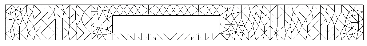
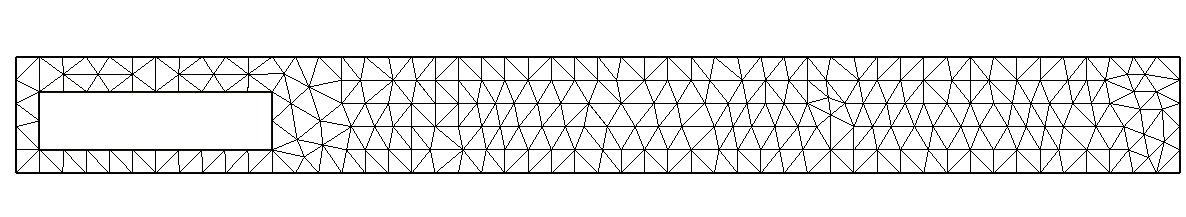
We start with an initial solution in which the hole is located at the bottom left corner of the beam:
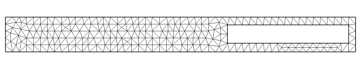
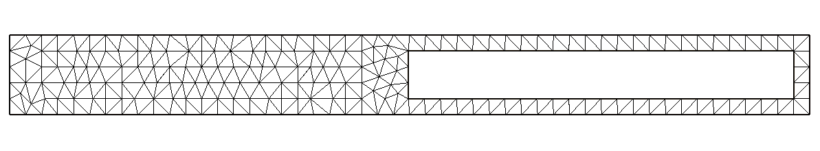
After 5 iterations, Hexaly has moved the hole to the right-hand side of the beam:
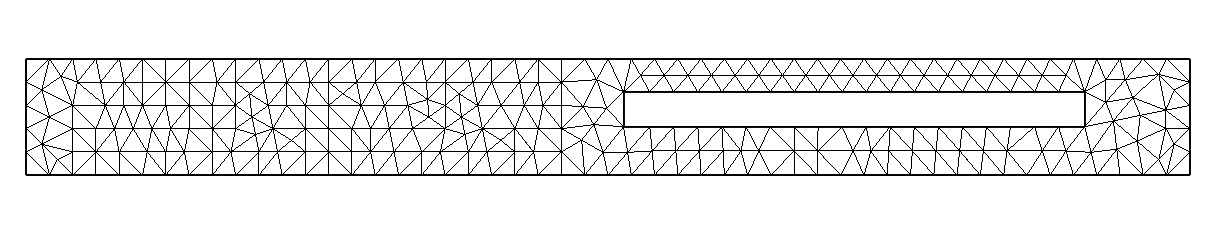
After 10 iterations, the hole is as close as possible to the top, right, and bottom boundaries of the beam:
After 50 iterations, the search has converged:
After 50 iterations, the best solution found is of excellent quality. As expected, the hole has moved to the right-hand side of the beam. Overall, writing and solving such a simulation optimization problem with Hexaly is very straightforward. Indeed, Hexaly was able to find this solution without information on the structure of the objective function. The user only has to tell Hexaly how to evaluate the objective function with the simulator.
The only bit of code specific to FreeFem++ in this example is the implementation of the get_compliance function. You can replay it by installing FreeFem++ and downloading the code here. You can also replicate this example with any other simulator able to communicate with Python (or C++, C#, or Java).
Are you interested in trying it out? Get free trial licenses here. In the meantime, feel free to contact us; we will be glad to exchange about your optimization problems.
[1] HECHT, Frédéric. New development in FreeFem++. Journal of numerical mathematics, 2012, vol. 20, no 3-4, p. 251-266.
Ready to start?
Discover the ease of use and performance of Hexaly through
a free 1-month trial, or enjoy free academic access.